SWE Lesson Series: First lesson posted
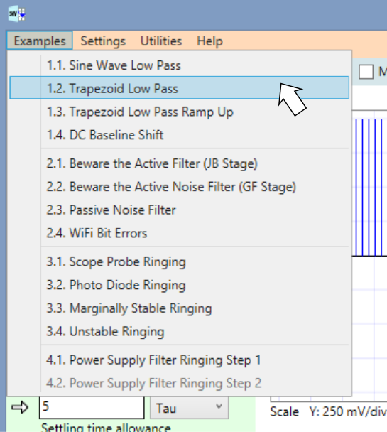
Included in Signal Wave Explorer are a set of canned examples that showcase the power of SWE in creating various types of circuit simulations. Many of these examples also illustrate common pitfalls that can trip up the unwary circuit designer. The examples cover a wide range of topics, starting with the basics, and working up to more complex scenarios. Here are the examples currently included in the product:
To go along with these examples, we are writing a set of papers that explain each of these examples in detail, both from a theoretical point of view and from an operational point of view — that is, how to set them up in SWE, and how to modify the parameters for further explorations.
Lesson 1.1. The Sine Wave Low Pass Example
We are pleased to announce that the first of these papers, covering the beginning lesson “Sine Wave Low Pass Example” is now available for download in PDF form. You can go to the download section to get your copy now, or simply click on the following link:
Lesson 1.1. Sine Wave Low Pass Example
In this post, we’ll summarize the things included in this first lesson, and paraphrase much of the discussion, which is about the use of an RC low pass filter, and what happens when you pass a sine wave through such a filter. We are giving lots of detail in this first in a series of blog posts to point out that there is a lot of information packed into these lessons! We encourage you to download them as they come online.
Continuous Analog Processing
From a continuous, analog point of view, the processing in the first lesson looks like:
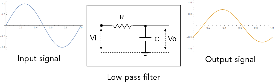
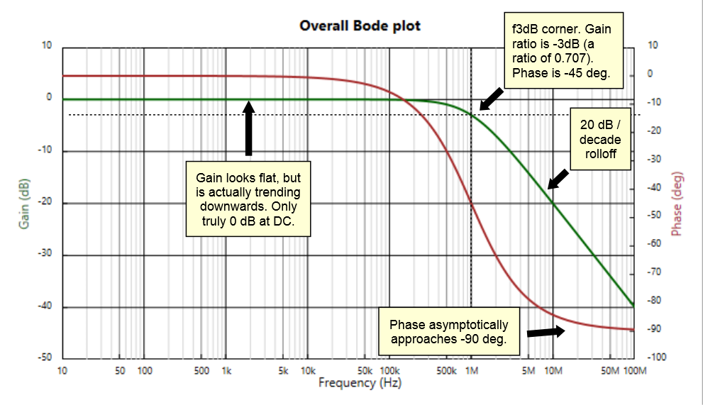
In our example, we’re using a 1 MHz sine wave with an amplitude of 1 V. We pass this through an RC filter having a 1 MHz corner. The filter reduces the amplitude of the sine wave, and causes a phase shift. Since our sine wave has exactly the same frequency as the filter’s corner frequency, those familiar with first order systems (like our RC filter) can recite from memory the corresponding gain and phase: 0.707 (1 / Sqrt 2) gain, -45 deg phase.
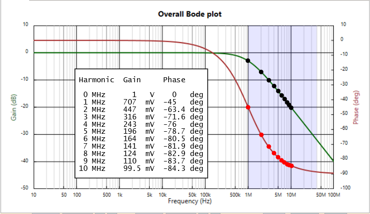
These numbers can be seen in a Bode chart representing the filter, as shown below, produced in SWE and annotated for our discussion here:
How can a person derive such a Bode chart? Well, by using the gain and phase formulas for an RC low pass filter. From a system point of view, the transfer function of an RC low pass filter is:
\(\displaystyle \frac{{{{V}_{o}}}}{{{{V}_{i}}}}=\frac{{{{Z}_{c}}}}{{R+{{Z}_{c}}}}=\frac{{\frac{1}{{j\omega C}}}}{{R+\frac{1}{{j\omega C}}}}=\frac{1}{{j\omega RC+1}}\)
Where
\(\displaystyle {{Z}_{c}}=\frac{1}{{j\omega C}}\)
is the complex impedance for a capacitor, and comes from the capacitor’s reactance — that is, how the capacitor reacts to sinusoids at different frequencies. The lower the frequency, the higher the impedance. The higher the frequency, the lower the impedance. At very low frequencies, the capacitor acts as though it’s an open circuit. At higher frequencies, it acts more like a short.
Note that our RC circuit is really a voltage divider in disguise, with a series resistance R and a shunt capacitance C with impedance Zc. From a voltage divider point of view, the ratio between voltage across the capacitor — which we treat as output voltage, to the input voltage — measured from the left side of the resistor to ground, can be written as:
\(\displaystyle \frac{{{{V}_{o}}}}{{{{V}_{i}}}}=\frac{{{{Z}_{c}}}}{{R+{{Z}_{c}}}}\)
and now you know how we derived the filter’s transfer function earlier. From that complex formula, with a bit of complex algebra (yikes for many of us!) you can represent the response in polar form — that is, as gain (the magnitude of the complex expression) and phase (the argument of the expression).
\(\displaystyle Gain(\omega )=\sqrt{{\frac{1}{{1+\mathop{{(\omega RC)}}^{2}}}}}\)
\(\displaystyle Phase(\omega )=-{{\tan }^{{-1}}}\left( {\frac{1}{{\omega RC}}} \right)\)
And this is where the Bode curves come from.
Sampled Time Domain Results
While SWE has the continuous form of the filter tucked away in its bowels, in performs simulations by using discrete samples. In our case, we are using 80 samples to cover one sine wave period. The input and output waves of our simulation look like:
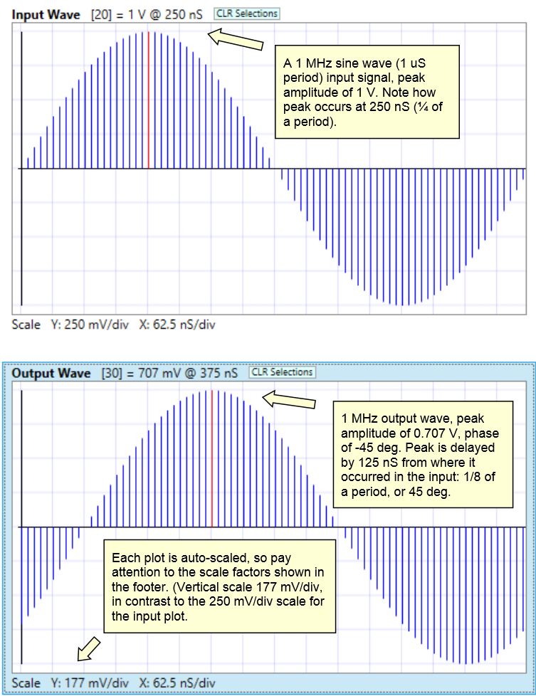
The output plot clearly shows the reduced amplitude of 0.707 V. The -45 degrees phase shift has to be deduced by seeing how much the peaks and zero crossings are delayed. In this case, by 1/8 of a period, or 360/8 = 45 degrees.
Input Spectrum in the Frequency Domain
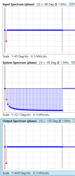
While SWE can show you results in the time domain, it’s using frequency domain processing underneath, in the form of Discrete Fourier Transforms. The input signal is transformed into the following magnitude and phase spectrums, as plotted in SWE:
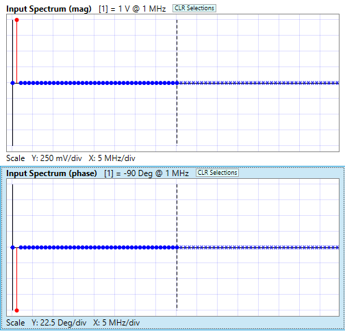
I know, not really exciting, since for a simple sine wave we have just one non-zero Fourier harmonic at the fundamental frequency (which in this case is 1 MHz). We’ve annotated that sample point in red on the plots above. You might wonder about the -90 degrees phase shift shown for the sine wave. What’s up with that? Well, you’ll have to read the lesson! Have fun!
System Response in the Frequency Domain
In SWE we represent the system response as a series of harmonics that are from points sampled on the Bode curves. To see how this is derived, below we show once again the Bode chart, but annotated with the first ten harmonic samples (plus DC, whose point isn’t shown).
Now, to create our system spectrum, we actually use 40+1 harmonic samples (1 MHz to 40 MHz, plus DC). Below are the spectrum plots produced in SWE for our 1 MHz low pass filter. We show the fundamental harmonic sample (at 1 MHz) in red:
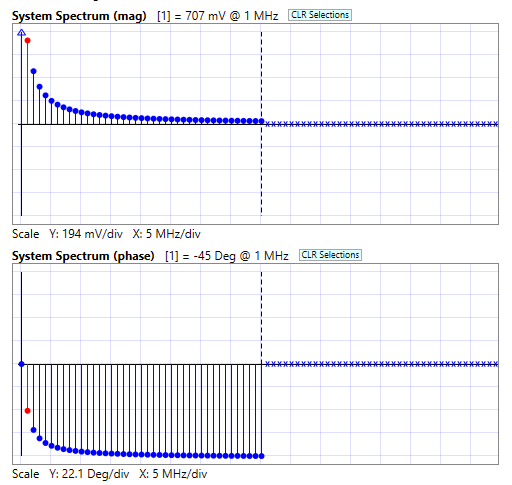
Now, these gain and phase curves look nothing like the continuous curves on the Bode chart, but they come from the same source. Why don’t they look the same? The Bode chart is log-log, the system spectrum plots are not. The spectrum plots only show samples in 1 MHz increments, plus a sample at DC.
You might wonder about the vertical dashed lines seen in the spectrums. They represent the location of the Nyquist frequency, which is half the sampling frequency. In our case, we use 80 samples, so the sampling frequency is 80x1MHz = 80 MHz, and the Nyquist frequency is 80/2 = 40 MHz. In the plots above, we are showing the spectrums as single-sided, and you are seeing the left side, from DC to 40 MHz. In the internal Fourier transform processing, there is also a right side that’s a conjugate-mirrored form of the left side. That’s right, the spectrums are actually double-sided — they have to be for the Fourier transforms to work correctly. For reasons beyond the scope of this blog post, we aren’t showing the mirrored side in the plots above, instead using x’s to stand for detail that is not given.
In case it hasn’t dawned on you, there’s lots of subtlety involved in doing the simulations, and SWE does its best to help you wade through the thickets.
The Output Spectrum
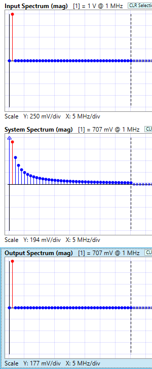
The compute the output spectrum, the input spectrum is multiplied, harmonic bin by harmonic bin, with the system spectrum, using complex arithmetic. The result is a spectrum that represents the output wave in the frequency domain. Below we show how the bins line up, ready for the complex multiplies to take place, using the samples in polar form (magnitude and phase). We take a sample from the input spectrum, complex multiply it by the corresponding sample from the system spectrum, and get back an output spectrum sample.
 |
 |
NOTE: For the complex multiplies, we are using polar form: multiplying the magnitudes and adding the phases. If a resulting sample has zero magnitude, we set the phase to zero as well, by convention. In our case, only one output sample has a non-zero magnitude, and thus there is only one non-zero phase.
Convolution Theorem is the Key
So why are we doing these multiplications in the first place? Well, as we mentioned in an earlier blog post, multiplication in the frequency domain equals convolution in the time domain. That’s in essence a statement of the convolution theorem, which is at the heart of how SWE is able to produce its results.
Back to the Time Domain
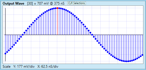
Now that we have an output spectrum, we can convert this whole mess back into the time domain, using an Inverse Discrete Fourier Transform. For our simple case here, we can do this “by inspection” by looking at the output spectrum plots. Note in the magnitude spectrum at bin 1 (the fundamental harmonic) we have an magnitude of 707 mV. That represents a 1 MHz sine wave (1 MHz is our fundamental frequency) with an amplitude of 707 mV. In the phase spectrum, we see phase of -135 degrees. Now, it turns out that in order to interpret this wave as a sine wave, we have to add 90 degrees to this number to get the proper phase shift. (Yes, this is the same curious 90 degrees we mentioned earlier.) So we end up with -135 + 90 = -45 degrees phase shift.
Well, waddya know! The output spectrum is predicting a 707 mV sine wave, at 1 MHz, with a -45 degrees phase shift. Why, that sounds familiar!
Now, ordinarily, to construct an output wave in general, we’d have to do what we just did for each harmonic sample. But in our case, there’s only one harmonic that has non-zero information, so we can just directly draw a sine wave using that information. Here is that output wave, in all its glory:
Like what you see?
Have we intrigued you yet? We hope so! We hope you’ll download this lesson and give it a read and do explorations in time and frequency using SWE. And if you haven’t downloaded SWE yet, you can get a trial version right now by following this link:
Comments
SWE Lesson Series: First lesson posted — No Comments
HTML tags allowed in your comment: <a href="" title=""> <abbr title=""> <acronym title=""> <b> <blockquote cite=""> <cite> <code> <del datetime=""> <em> <i> <q cite=""> <s> <strike> <strong>