We are pleased to announce the addition of another lesson in the SWE Lesson Series, this one on low-pass-filtered trapezoid signals. It’s available in PDF form on the Downloads Page, or you can get it directly from the following link:

Lesson 1.2. Trapezoid Low Pass Example

We’ll be adding a series of blog posts in the next few days that highlight various sections of this lesson, in a category of articles we call “Short and Sweet.” We’re developing a new section on this website for these Short and Sweet articles, which are intended to be little snippets of math and theory and practical considerations related to circuit design, and to the use of our products.

Examples to Whet Your Appetite

Here are a few of the images found in Lesson 1.2, to whet your appetite.

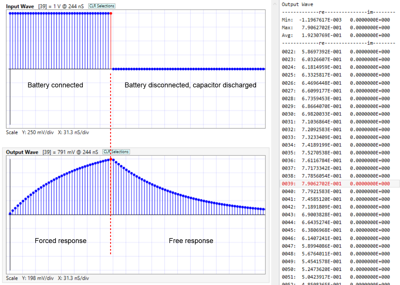
This one shows the default output when you run the simulation:

This one shows a capacitor charging/discharging circuit:

 

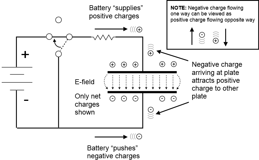
that we model using a square wave pulse:

Here, we compare the results obtained by SWE simulation with that predicted from the analytical equations:

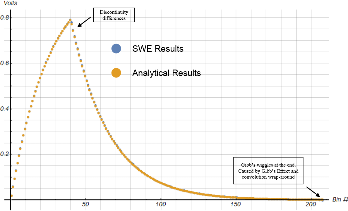
Simulations using Discrete Fourier Transform processing, like we’re using in SWE, are subject to small artifacts known as the Gibb’s Effect, and convolution wrap-around. Here’s an example where we’ve zoomed in at the end of the previous plot:

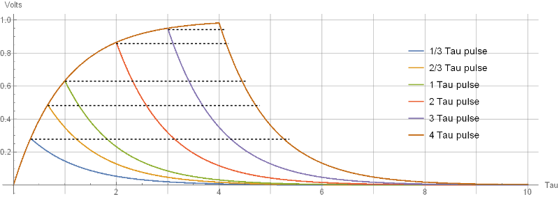
This plot illustrates how input pulses of various widths, have the same exponential curves on output, both for charging and discharging. They just stop charging at different points, and then start discharging, using the same exponential decay. The input pulses (not shown by the way), are represented in terms of “tau widths”. That is, their widths are in units relative to the time constant of the low pass filter.

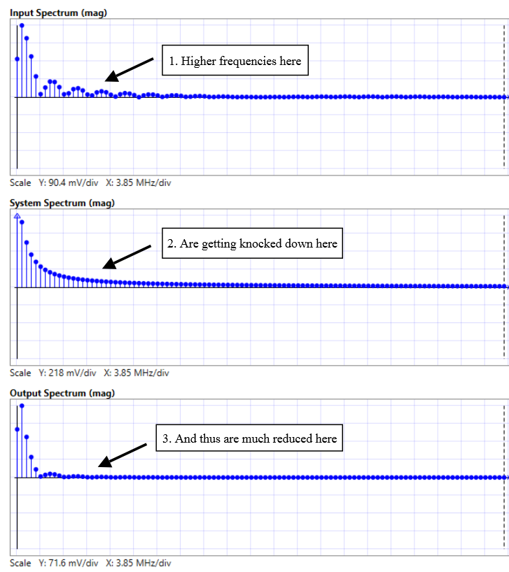
Next, we have an illustration showing how to view signal processing calculations in the frequency domain. Here, we plot the spectrum of an input trapezoid wave, (plus zero-padding for the simulation), and then shown the corresponding system spectrum, which comes from sampling the low-pass filter response, and then resulting output spectrum, which can be obtained by multiplying the input and system samples, bin by bin. Here, we’re showing only the magnitude portion of the spectrum.

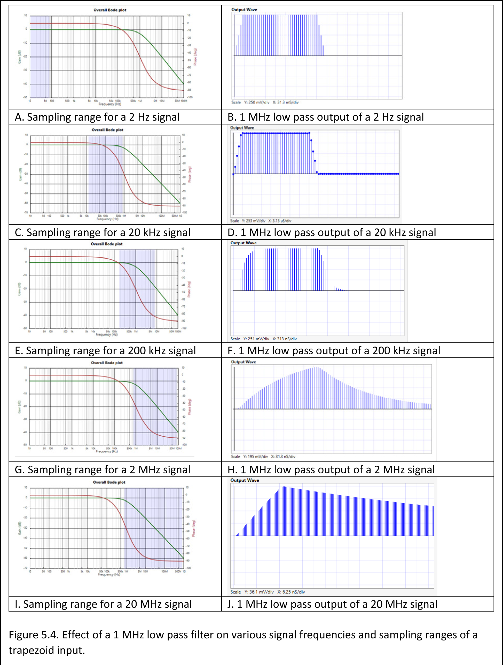
This next image illustrates a cool feature of SWE. You can see the simulation sampling range right on the system bode chart. (It’s the blue overlay.) This gives you an idea of what the system will do to your signals. For example, if the curve covering the sampling range is all flat, then the signal is going to pass through pretty much unchanged. If however, the range starts encroaching on the f3dB corner frequency of the filter, or down the -20db/decade slope, then the high frequency “corners” of the signal will get softened in the time domain:

There’s much more in the lesson example, which you can download in PDF form using the following link:

Lesson 1.2. Trapezoid Low Pass Example