Time Domain Simulations Using Fourier Transforms
Our new product, Signal Wave Explorer (SWE), gives you the ability to run circuit simulations and predict output waveforms. Those of you familiar with Spice tools might think we are doing these simulations using some version of Spice. But we’re not — and that’s what makes us unique.
So how are we doing things? By using code developed here at Robust Circuit Design that utilizes Fourier transforms. To illustrate this, we’ve developed a 124 slide presentation that you can download in PDF form from the following link:
Time Domain Simulations Using Fourier Transforms
This presentation is also included as part of the SWE Product Download.
In this post, we’ll be highlighting some of the things you can learn from the slide presentation.
How is SWE Different?
What does SWE do that’s different from what Spice does? Essentially, Spice does its magic by solving matrices at runtime. These matrices represent the simultaneous differential equations that define the behavior of the circuit being simulated. Spice is using numerical integration, and for the most part, it’s doing its processing, both of any signals and the circuit itself, in the time domain.
In contrast, SWE does its magic by processing both signal and system in the frequency domain, yet taking time-domain input signals and producing time-domain output signals. Why use the frequency domain for processing? It’s due to historical reasons that came about during the development of the sister product, Signal Chain Explorer (SCE).
SCE was designed to use the gain and phase response curves constructed for arbitrary linear signal chains. It uses these curves along with parasitic and noise interference analysis to compute signal-to-noise ratios — gargoyles as we call them in SCE. Determining the quality of the signal is paramount to SCE and that’s why the single signal-to-noise ratio is important. But we kept thinking as we developed the product,
“How cool it would be to show, for any input, how the output looks in time, noise and parasitics and all?”
Could we pull this off? SCE does not use any time-domain equations underneath. All it has to work with is the gain and phase curves of the overall system — information that’s entirely in the frequency domain.
That’s where Fourier transforms come in to play. We recognized that these would allow us to take a time domain signal, transform it into the frequency domain, do some processing, and then transform the result back into time. A few months of research and development later, and we had the ability to do just that. That’s how SWE was born. It served originally as a test bed for technology that we hope will later make its way into SCE, and we decided that SWE would be a good product in its own right.
Convolution Illustrated
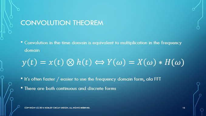
SWE works by taking advantage of an important theory of convolution:
Convolution in the time domain = multiplication in the frequency domain
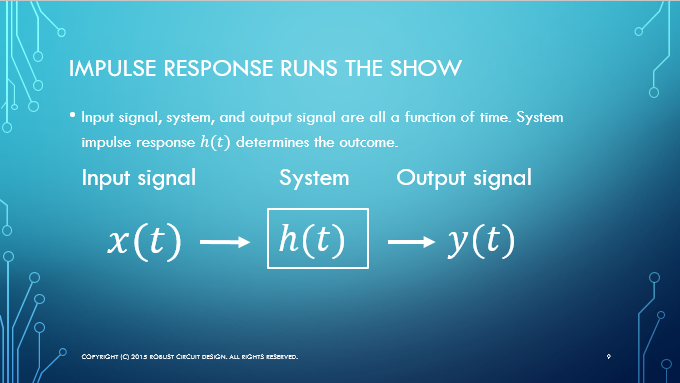
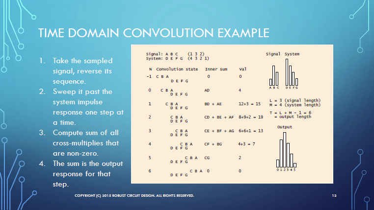
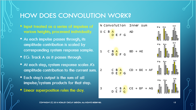
Now, what’s all this talk about convolution? It’s part of the theoretical underpinnings of signal processing. Think of convolution as a sort of reverse cross-correlation of input signal and system response. The input signal is convolved with the system’s impulse response to produce an output response. Here are a few slides borrowed from the presentation that illustrate what convolutions are all about.
Now, this is all fine and dandy, but it’s in the time domain. As we mentioned earlier, SCE only works in the frequency domain. So what to do? Well, the Convolution Theorem came to our rescue. We restate this theorem below, as given in the presentation:
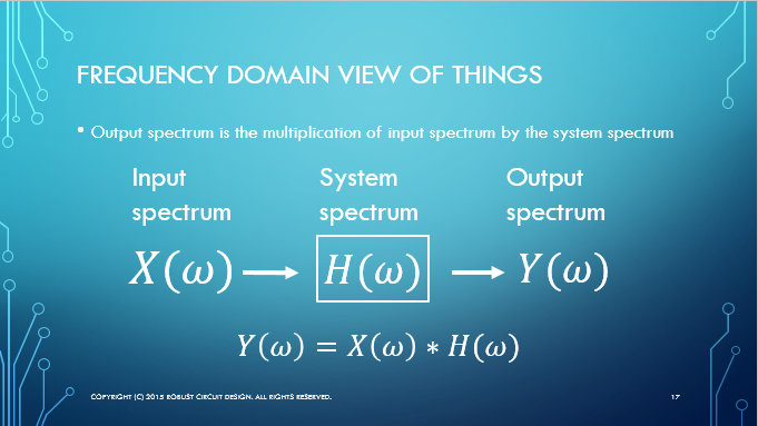
To the Land of Frequency and Back
SWE takes an input signal, converts it into the frequency domain using a Discrete Fourier Transform (DFT)*, multiplies this computed spectrum with the system response spectrum in the frequency domain, gets an output signal in the frequency domain as a result, and then converts this output spectrum back into the time domain, using an Inverse Discrete Fourier Transform (IDFT).
* By discrete, we mean SWE takes samples of the input signal, as well as the system response. The resulting output is sampled as well.
Input signal spectrum
Here’s an illustration of the first part of processing SWE does, using a trapezoid wave. We’ve taken 208 samples of the trapezoid, and then transformed the wave into its magnitude and phase spectrum counterparts (only a portion of the samples are shown):

System Spectrum Secrets Revealed
We must multiply the input spectrum by the system’s response spectrum. We know the system’s continuous gain and phase curves, but how do we get this in a sampled form suitable for multiplying with the input signal?
This question stumped us for quite some time, because here’s the kicker: We could not find anywhere on the web a description on how to do this with enough detail to actually implement it.
That’s not to say there weren’t plenty of sources that mentioned the idea in passing, but we found actual, live examples were few and far between, other than those that used analytical formulas to represent the system. The problem is, in SCE (and SWE) we in general don’t know the system response in analytical form. All we have are the derived gain and phase curves of a signal chain composed from numerous stages.
We finally cracked this secret — and lucky you — it’s revealed in the accompanying slide presentation. The SWE User’s Manual included in SWE also provides details. And we encourage you to download the SWE Trial Version to see this in action for yourself.
For now, we’ll give you an idea of what such a sampled spectrum looks like. Here is the magnitude and phase spectrum for a 1 MHz low pass filter. Again, we are only showing a portion of the samples, and do note our spectrum plots are linear in the Y-axis:
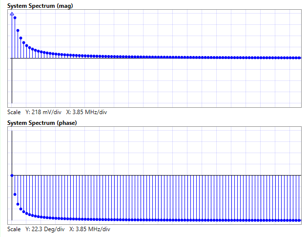
Each sample in the plots represents the magnitude and phase, respectively, for a given frequency. The zeroth sample, called Bin 0, represents the DC gain and phase. Bin 1 gives the response for a frequency that’s equal to the fundamental frequency (first harmonic) of the input signal. Bin 2 gives the response for the frequency of the second harmonic, and so on. To do the processing, SWE takes samples from the input spectrum and multiplies them, bin by bin, with the samples from the system spectrum. Complex multiplication is used. The resulting spectrum represents the output signal in the frequency domain.
Here’s an example of the output spectrum for our case here, followed by the time domain wave that we obtain by taking an Inverse Discrete Fourier Transform:
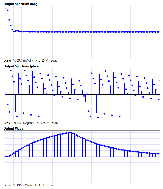
We basically get the classic exponential ramp-up and decay of a first order system, here for the case when a trapezoid signal is the input. Pretty cool, eh?
Are you itchin’ to try it?
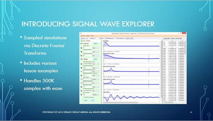
As summarized in the slide presentation, SWE has the following features:
Have we piqued your curiosity? Don’t you want to try this now?
Comments
Time Domain Simulations Using Fourier Transforms — No Comments
HTML tags allowed in your comment: <a href="" title=""> <abbr title=""> <acronym title=""> <b> <blockquote cite=""> <cite> <code> <del datetime=""> <em> <i> <q cite=""> <s> <strike> <strong>