In the last Short and Sweet article we talked about the input and output impedances of inverting and non-inverting op-amp stages. We sort of jumped the gun a little, because we never mentioned exactly what is meant by input and output impedance. In particular, we didn’t really explain what local impedance is. In this (not so) Short and Sweet article, we’ll do just that.

NOTE: The term local impedance is something we invented here at Robust Circuit Design. You’re not likely to find that terminology anywhere else. Local impedance simply means “the input or output impedance of a stage in a signal chain as though that stage is the only stage.” That is, we treat the stage in isolation when measuring the impedance.

First Principles

We’ll start by defining ordinary input and output impedance. We refer you to the diagram below.

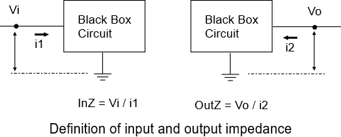
Suppose you have a circuit that to you is a “black box” — you don’t know what’s inside, other than knowing that any voltage sources contained therein are set to zero volts, and any current sources are opened. Suppose the black box has a single input that you can inject a small current into and that you can then measure the resulting voltage at the input, referenced to circuit ground. Alternatively, maybe you apply a voltage and measure the corresponding current. Either way, with voltage and current in hand, the input impedance of that circuit can be calculated using Ohm’s Law:

\(\displaystyle InZ=\frac{{Vi}}{{i1}}\)

If your circuit is used as a load to another circuit, then that other circuit sees this much impedance as its load impedance.

Suppose the black box circuit has a single output (besides ground). You could inject a small current back into that output and measure the resulting voltage referenced to the circuit ground. Or alternatively you might apply a voltage and measure the corresponding current. Either way, with voltage and current in hand, the output impedance can be calculated using Ohm’s Law:

\(\displaystyle OutZ=\frac{{Vo}}{{i2}}\)

If this circuit is used as a source to another circuit, then that other circuit sees this much source impedance.

To summarize, when connecting circuits together, input impedance can become load impedance, and output impedance can become source impedance.

Your black box circuit might contain both resistive and reactive components, so the input and output impedances are in general complex variables. This means the impedances can vary by frequency.

Impedances in a signal chain

A signal chain is a series of sub-circuits arranged in a linear fashion, where a signal flows from left to right. We call the sub-circuits stages, and the first stage is normally a sensor of some kind. Here’s a diagram illustrating this:

In analyzing the behavior of a signal chain, it can be useful to know the input (or output impedances) at any given stage. Knowing those impedances helps us understand how the signal chain behaves at that point.

Input Impedance at a given stage

Suppose you want to know the input impedance at stage N. As illustrated below, in determining the input impedance, you must not only consider any impedances in stage N itself, but all the stages that follow:

How do we go about doing this? Well, we could find the input impedance to stage N+1, and treat that as a “load” to stage N. For example:

We mentioned this idea earlier, that the input impedance of one stage can become the load impedance of another.

How do we find the input impedance of stage N+1? Well, we find the input impedance of stage N+2 and treat that as the load for stage N+1. Put that in your pipe and smoke it!

Input impedance of the last stage

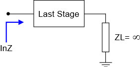
We can continue this inductive process until we reach the last stage. Then we reach a boundary condition. What is the load of the last stage? Mathematically, it’s a load with infinite input impedance:

Input impedance of single stages

The boundary condition used in computing the input impedance of the last stage can also be used to treat any stage in isolation. We pretend the other stages don’t exist. Next, we’ll look at three specific but simple cases to help you understand how this works. The three cases we consider are: (1) a series stage, (2) a shunt stage, and (3) a voltage divider stage.

Input impedance of a series stage

We’ll start with a signal chain that consists solely of a series impedance Zs:

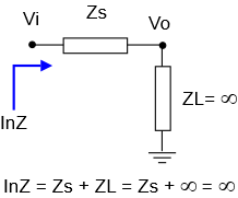
Our single stage, being by definition the last stage, has an implied load of infinite impedance. So what’s the total input impedance? To someone looking in from the left, it looks like an impedance Zs in series with an infinite load impedance. The end result is that the input impedance is infinite!

Can this be true? Well, a series stage all by itself is “floating”. In such a circuit, no current can flow. If this floating stage itself were to be treated as a load to another stage, since no current flows through this newly designated load, that’s the same as saying it too has infinite impedance.

Input impedance of a shunt stage

Next, we consider a shunt stage Zs all by its lonesome. Being again the last stage by definition, it’s in parallel with a load of infinite impedance:

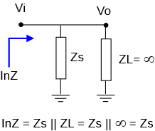
To someone looking in from the left, all the input current flows through Zs, since none can flow through ZL with its infinite impedance. Thus, the input impedance of a shunt stage is the impedance of the shunt itself. We note mathematically:

\(\displaystyle Zs||ZL=\frac{{Zs\,ZL}}{{Zs+ZL}}\)

and

\(\displaystyle \underset{{ZL\to \infty }}{\mathop{{\lim }}}\,\frac{{Zs\,ZL}}{{Zs+ZL}}=Zs\)

Input impedance of a voltage divider

Next, we look at a voltage divider as our sole stage. As before, we tack on the implied infinite impedance load:

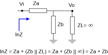
What’s the input impedance of this stage? Any current flowing into this stage has only one way to go: through Za and Zb. No current will flow through ZL with its infinite impedance. Thus, this stage looks like Za in series with Zb.

More complicated stages

With our simple single-stage examples, you should now begin to understand how input impedance is found. Obviously more complicated stage examples could be considered, but that’s too much detail for this supposedly Short and Sweet article. But the notion of looking at series and parallel branches, and/or voltage dividers, all tacked on with an “infinite” load impedance, is the basic trick to remember.

There is, however, another concept to learn that’s directly related to our single stage configuration: local input impedance.

Local input impedance

The local input impedance of a stage is defined as the input impedance the stage would have if were the only stage in the signal chain. In other words, it’s the impedance the stage would have if it were the last stage. To repeat:

DEFINITION: Local input impedance = input impedance as if the stage were the last stage

Here’s a diagram illustrating this:

To recap what we learned earlier about our simple single stages and how that now relates to local input impedance, we can say:

\(\displaystyle \text{Local InZ of series stage}=\infty \)

\(\displaystyle \text{Local InZ of shunt stage}=Zs\)

\(\displaystyle \text{Local InZ of voltage divider}=Za+Zb\)

Input impedance with Signal Chain Explorer

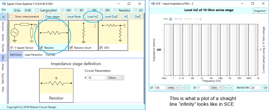
Next, we look at how to find the input impedance of any stage in an SCE signal chain. Below is an arbitrary signal chain having various stages, the first of which is a 10 Ohm series resistor stage. The left diagram shows how the series stage is selected and where to push the Local InZ button. The plot on the right is the impedance vs frequency, which in this case is just a (missing) straight line, at infinity.

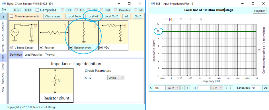
Here’s the same kind of thing for a 10 Ohm shunt stage. The plot shows a straight line at 10 Ohms.

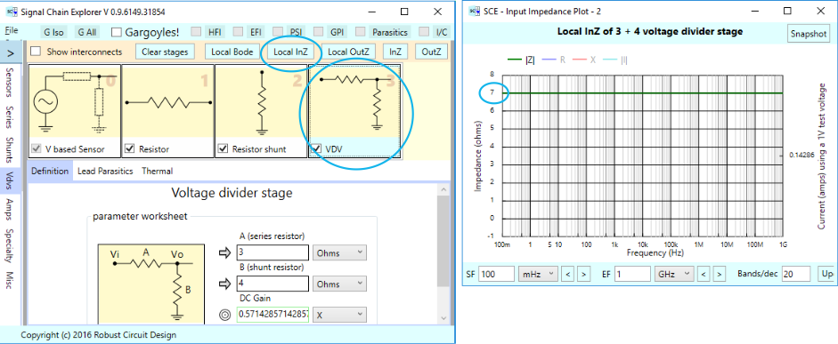
And then we have a voltage divider stage, with a series branch of 3 Ohms and shunt branch of 7 Ohms. The plot once again shows a straight line — this time at 3+4 = 7 Ohms.

Just to remind you that impedances can be complex and vary with frequency, here’s a passive band-reject filter and it’s associated local input impedance plot:

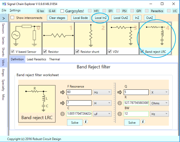
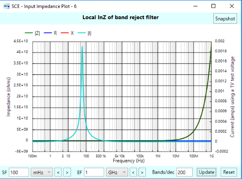
We have a rise in current (the turquoise line) at 60 Hz, which represents the shunting of current to ground, as by design of the stage. (The notch resonance was configured to be 60 Hz.)

This figure illustrates why we also show current on the impedance plots. The turquoise line represents the current as if a voltage of 1 V were applied at any given frequency. Due to the (linear) scale of the plot, we can’t see that the reactance is going to zero right at resonance, (which causes the current to peak), because the impedance itself shoots towards infinity at higher frequencies. But the current line is giving us a hint that something is going on at 60 Hz.

Without getting too detailed about this (we’ll save that for a later article), we can zoom in to see what’s happening. Here, the red line is reactance, the blue line resistance, and the green line the magnitude of the impedance:

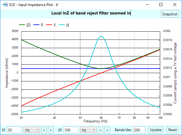
Let’s look at this mathematically. The local input impedance of this stage is comprised of a resistor, inductor, and capacitor all in series, so:

\(\displaystyle \text{Local InZ of band reject}=R+j(\omega L-\frac{1}{{\omega C}})\)

The reactance (imaginary) term goes to zero when the terms involving L and C cancel out, which occurs right at 60 Hz in our case. The overall impedance doesn’t go completely to zero, however, because of the series resistance R. That’s why the current peak is rounded. As the frequency rises past resonance, the L term takes over, and the overall impedance goes up and up, theoretically to infinity, as you saw in the zoomed out plot.

ddda0da3-523098562 3-5409238 5-0239582 3-059238 5-023985 23-095823 -059823 098

Output Impedance at a given stage

Let’s switch gears and look at output impedance. Suppose you want to know the output impedance of stage N. As illustrated below, in determining the output impedance, you must not only consider any impedances in stage N itself, but all the stages that precede it:

How do we go about finding this? Well, we could find the output impedance of stage N-1, and treat that as the “source” to stage N. For example:

We mentioned this idea earlier, that the output impedance of one stage can become the source impedance of another.

How do we find the output impedance of stage N-1? Well, we find the output impedance of stage N-2 and treat that as the source for stage N-1. Put that in your pipe and smoke it!

Output impedance of the first stage

We can continue this inductive process until we reach the first stage. Then we reach a boundary condition. What is the source impedance of the first stage? In SCE, the first stages are always sensor stages. Below, we’ve represented the sensor generically as an ideal voltage source along with a series impedance Zs. That impedance is the output impedance for the stage.

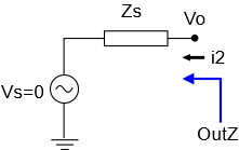
NOTE #1: Of course, more complicated sensor scenarios exist that we won’t go into here. And we note that in the case of current source sensors, we can just convert to the Thevenin equivalent.

NOTE #2: In keeping with how impedances are determined, we set the sensor voltage to zero when finding the output impedance.

Suppose the sensor has no series impedance. Then what impedance do we use for the stage? Well, we have the ideal voltage source, which by definition has an output impedance of zero.

NOTE: If you use a current source for your sensor, then it may be of interest for you to know that the output impedance of an ideal current source is infinite.

Output impedance of single stages

If we wanted to find the output impedance of a signal chain having only one stage and that stage wasn’t a sensor, then what do we do? Merely pretend that the stage has an ideal voltage source attached to it, as we show below. The source impedance coming in to our stage is thus zero.

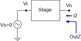
As always, we must set the voltage of the source to zero in order to find the stage impedance.

Note the symmetry between input and output impedance: For input impedances, the last stage has an implied load with infinite impedance. For output impedances, the first stage has an implied voltage source in front of it, (that we set to zero), with zero impedance. This is summarized in the following diagram, which we show for a signal chain having only one stage:

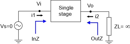
Next, we’ll look at three specific but simple cases to help you understand how this works. The three cases we consider are: (1) a series stage, (2) a shunt stage, and (3) a voltage divider stage.

Output impedance of a series stage

We’ll start with a signal chain that consists solely of a series impedance Zs:

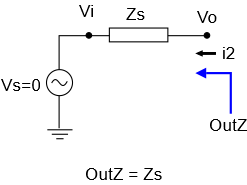
Our single stage, being by definition the first stage, has an implied voltage source of zero impedance. So what’s the total output impedance? To someone looking in from the right, it looks like an impedance Zs in series with a zero source impedance. The end result is that the output impedance is the impedance of the stage itself.

Output impedance of a shunt stage

Next, we consider a shunt stage Zs all by its lonesome. Being again the first stage by definition, it’s in parallel with a voltage source having zero impedance:

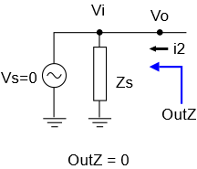
To someone looking in from the right, all the current flows through the voltage source branch, since it’s a short! So the output impedance is zero.

Output impedance of a voltage divider

Next, we look at a voltage divider as our sole stage. As before, we stick an ideal voltage source on the front:

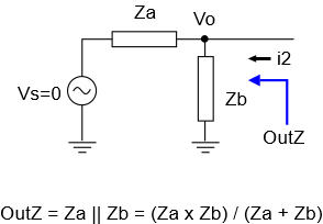
What’s the output impedance of this stage? Any current flowing into this stage from the right has two pathways to ground: through Za and Zb. That is, we have a parallel configuration. So the output impedance is the parallel impedance of the two branches.

More complicated stages

With our simple single-stage examples, you should now begin to understand how output impedance is found. Obviously more complicated stage examples could be considered, such as a closed-loop amp stage, which we’ll see later. In general, though, it’s too much detail for this Short and Sweet article, but the notion of looking at series and parallel branches, with a zero source impedance tacked on front, is the basic trick to remember.

There is, however, another concept to learn that’s directly related to our single stage configuration: local output impedance.

Local output impedance

The local output impedance of a stage is defined as the output impedance the stage would have if were the only stage in the signal chain. In other words, it’s the impedance the stage would have if it were the first stage. To repeat:

DEFINITION: Local output impedance = output impedance as if the stage were the first stage

Here’s a diagram illustrating this:

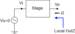
To recap what we learned earlier about our simple single stages and how that now relates to local output impedance, we can say:

\(\displaystyle \text{Local OutZ of series stage}=Zs\)

\(\displaystyle \text{Local OutZ of shunt stage}=0\)

\(\displaystyle \text{Local OutZ of voltage divider}=\frac{{Za\,Zb}}{{Za+Zb}}\)

Output impedance with Signal Chain Explorer

Next, we look at how to find the output impedance of any stage in an SCE signal chain. Below is an arbitrary signal chain having various stages, the first of which is a 10 Ohm series resistor stage. The left diagram shows how the series stage is selected and where to push the Local OutZ button. The plot on the right is the impedance vs frequency, which in this case is just a straight line at Zs = 10.

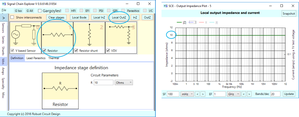
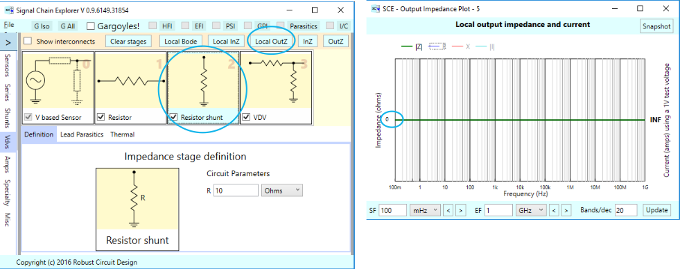
Here’s the same kind of thing for a 10 Ohm shunt stage. The plot shows a straight line at 0 Ohms.

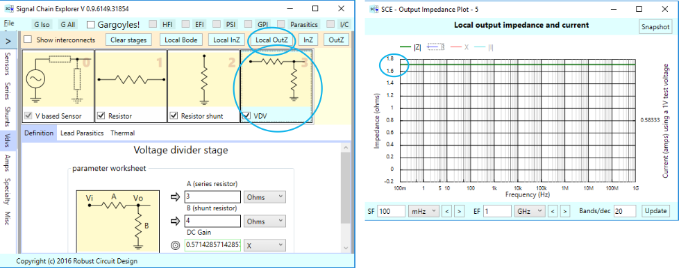
And then we have a voltage divider stage, with a series branch of 3 Ohms and shunt branch of 7 Ohms. The plot once again shows a straight line — this time at (3 x 4) / (3 + 4) = 1.714 Ohms.

Just to remind you that impedances can be complex and vary with frequency, here’s a passive band-reject filter and it’s associated output impedance plot:

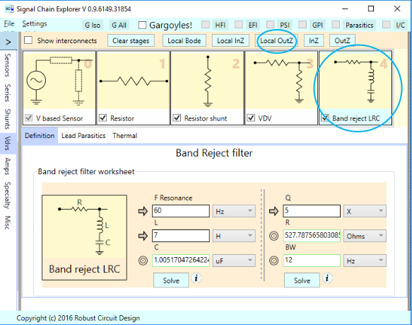
We have a notch right at 60 Hz, as by design of the stage. (F resonance was set to 60 Hz.)

Op-amp stage local output impedance revisited

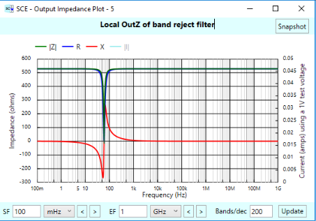
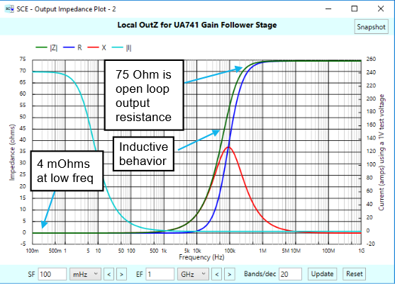
In the last Short and Sweet article we discovered that the local output impedances of a gain follower (aka non-inverter) and an inverter stage were identical, given the same amplifier and the same external resistance values. To refresh your memory, here are the two plots:

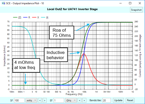
To see why this is so, reconsider the definition we gave for local output impedance: It’s the output impedance the stage would have if it were the first stage. Being the first stage, it’s implied that there’s a voltage source in front, with zero voltage and zero impedance. For a gain follower stage, that voltage source is driving the positive pin of the op-amp. For an inverter, it’s driving the negative pin. In both cases, the non-signal pin goes to ground. It’s possible to draw both of these stages using the same circuit topology but with a different signal orientation, and in doing so, we’ll also put in these voltage sources that are set to zero:

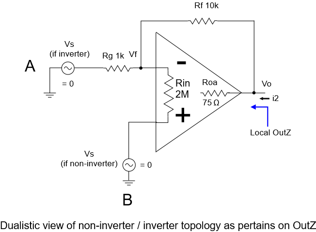
If A is the signal line, then we have an inverter. If B is the signal line, we have a non-inverter (gain follower). Either way, when we determine local output impedance, we set the associated voltage sources (the “signals”) to zero, and you can see by inspection that we have the same circuit. That means the local output impedances will be the same.

Just in case you want to know what that local output impedance is, here’s the formula in all its glory, where G(jω) is the open-loop gain of the op-amp, which varies by frequency:

\(\displaystyle LocalOutZ=\frac{{(Rf\,Rg+Rf\,Rin+Rg\,Rin)Roa}}{{Rf\,Rg+Rf\,Rin+Rg\,Rin+G(j\omega )Rg\,Rin+Rg\,Roa+Rin\,Roa}}\)

That varying open-loop gain serves to give the amp stages an inductive behavior on the output at intermediate frequencies.

Summary

You’ve seen how to think about input and output impedances, particularly as they pertain to linear signal chains. And you’ve been introduced to the concept of the local input and output impedance of a stage, which is derived by pretending the stage is the only one in the signal chain. Summarizing, local input impedances are found by setting the load of the stage to have infinite impedance. Local output impedances are found by setting the source of the stage to have zero impedance. We repeat a diagram we gave earlier to help you remember:

Armed with this knowledge, you are now ready to explore signal chains in Signal Chain Explorer and see what sort of mysteries you can uncover by examining the interactions between the stages, by way of both local and overall impedances. With Signal Chain Explorer, visualizing these impedances takes just a single click.