In Part 1 of this Short and Sweet article we derived the formula for thermal noise as it applies to RC filter circuits:

\(\displaystyle {{\eta }_{v}}^{2}={{KT}}/{C}\;\)

In this blog post, we’ll try out various RC filters using Signal Chain Explorer and see if this formula holds. While the formula was developed for low pass RC filters, it also works for other first order RC configurations as you’ll see.

Putting SCE to the test

Below is a screenshot of a signal chain we created in SCE consisting of a sensor (just a voltage source) and a low pass filter stage. For illustration purposes, we’ve set up a simulation frequency range of 100 mHz to 1 GHz, and we are purposely using a coarse simulation resolution of 2 bands/decade. For our filter, we’re using R = 10 Ohms, and C = 10 pF.

This filter has a corner frequency of 1.59 GHz as shown in the low pass filter worksheet. It also has an effective noise bandwidth (not shown) of:

\(\displaystyle {{f}_{{enbw}}}=\frac{1}{{4RC}}=\frac{1}{{4\times 10\times 10\times {{{10}}^{{-12}}}}}=2.5\,GHz\)

When we press the main Update button , SCE computes the integrated thermal noise of our filter and comes up with 15.1 uVrms, as indicated on the screenshot. Is this correct?

Well, from the KT/C formula, we can compute the theoretical amount:

\(\displaystyle {{\eta }_{v}}=\sqrt{{\frac{{KT}}{C}}}=\sqrt{{\frac{{1.38064852\times {{{10}}^{{-23}}}\times 290}}{{10\times {{{10}}^{{-12}}}}}}}=20\mu Vrms\)

NOTE #1: In case you are wondering, thermal noise voltage is specified as an RMS value. That’s because it’s actually a statistical value, as we noted in Part 1.

NOTE #2: SCE defaults the ambient temperature used in noise calculations to 290 degK.

Hmm, 20 != 15.1. Seems like SCE is plain wrong. Guess we should just delete the program off our system.

Please don’t do that! It’s only wrong because we didn’t use it right. And two wrongs don’t make a right. But what are the two wrongs?

1. We didn’t use enough resolution in our simulation, as indicated by the lowly 2 bands/decade. We’ll get back to that in a bit.
2. The reported thermal noise is the total integrated noise voltage over whatever frequency range we happened to pick for the simulation — in this case, 100 mHz to 1 GHz. But we didn’t cover a wide enough frequency range. We know this because the corner frequency for our filter is 1.59 GHz, and we’re only going out to 1 GHz. Not to mention the fact that we already know that the effective noise bandwidth is 2.5 GHz, and we haven’t covered that either. In fact, we’ll have to go out much further than the effective noise bandwidth. We can see this if we pull up the thermal noise plot by clicking the icon to the right of the overall thermal noise value on the main screen:

 

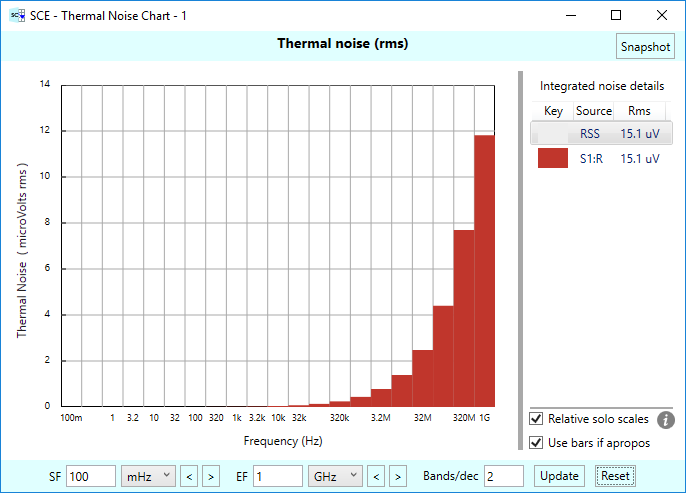
This is a plot of the thermal noise voltage by frequency “bands.” For each band, we compute the thermal noise for each noise source using the formula \(\displaystyle {{\eta }_{v}}=\sqrt{{4KTBR}}\), and for B we use the bandwidth of the band. Then, reminiscent of Part 1, we sum up those individual noises and come up with an integrated value.

NOTE: See Understanding SCE Thermal Noise Charts for more detail on how the thermal noise plots are produced.

The thermal noise plot is log-linear: the horizontal frequency axis is logarithmic, and the vertical noise voltage axis is linear. Because of the logarithmic scale, each band covers a progressively wider range of frequencies, as we go up in frequency. And a wider band means more noise. That’s why the plot is rising, even though as we noted before, thermal noise is “white”, and has a flat spectrum (if not filtered). That flatness is only true if the spectrum is shown linearly, rather than logarithmically as is done here.

From the rising plot we get the hint that maybe we aren’t seeing all of the thermal noise, and that’s a problem. For the integrated noise voltage computed, (the area under the curve so to speak), SCE uses only the frequency range selected — in this case from 100 mHz to 1 GHz. Let’s see what happens if we go out to a 100 THz instead. (Hey, this is math. We can do whatever we want! 🙂

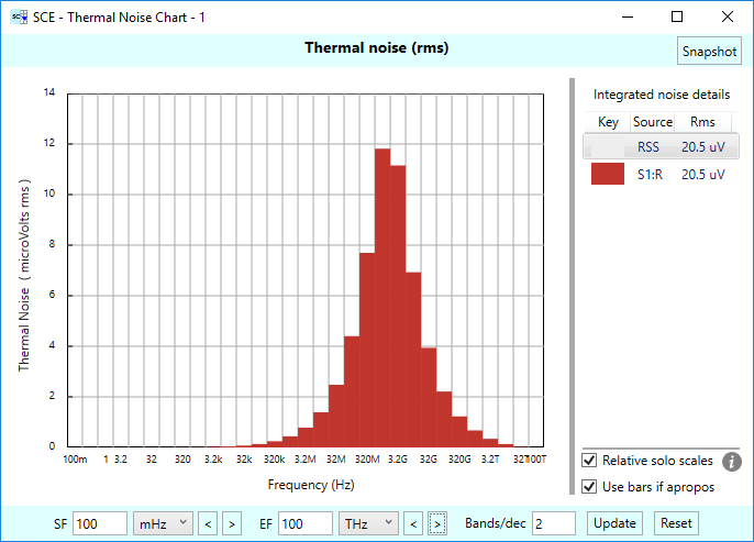
Looks like we’re covering an adequate frequency range now — we seemed to have captured all of the noise. So now our total integrated noise comes out to 20.5 uVrms, as indicated in the top right-hand corner of the plot.

Better. But 20.5 uV still doesn’t equal 20 uV, our theoretical number. Is the theory wrong? Is SCE simply not accurate enough? Nope on both counts. As you might have guessed from our rather coarse plot, we need to give the simulation more resolution. Let’s see what happens if we change the bands/decade from 2 to 20:

Now we get our fabled 20 uV. Yay!

NOTE #1: Our plot only reports a few significant digits in its results, so we may not be exactly at 20 uV, but it’s close enough for demonstration purposes.

NOTE #2: In case you are wondering, the thermal noise plots are showing noise voltage, and not noise power as we saw in Part 1 when we derived the KT/C formula. Also, the noise power plots were linear, whereas our thermal noise plots are log-linear. Because of these two reasons, the shapes of the two plots don’t come out the same. Not to worry, for we are indeed doing a integration of sorts when we compute thermal noise. We are adding up the noise voltages in all the bands, using a root-sum-square approach.

Reminder: For more information on how the thermal noise plots work, see the blog post we mentioned earlier: Understanding SCE Thermal Noise Charts.

Other RC circuits

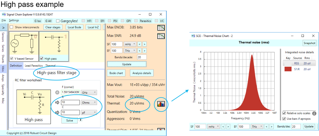
So you’ve seen that the KT/C formula works for low-pass RC filters, and we’ve confirmed it in SCE. But what about high-pass RC filters? What about parallel RC filters? We can construct such filters in SCE and find out! That’s what Signal Chain Explorer is all about — exploring. We’ll use the same R and C values as before, and we’ll use the 100 mHz to 100 THz frequency range that we settled on earlier, along with 20 bands/decade. The results for these other filter configurations are summarized in the following figures:

Parallel RC version

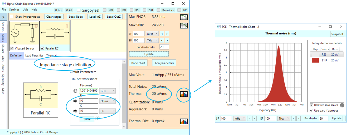
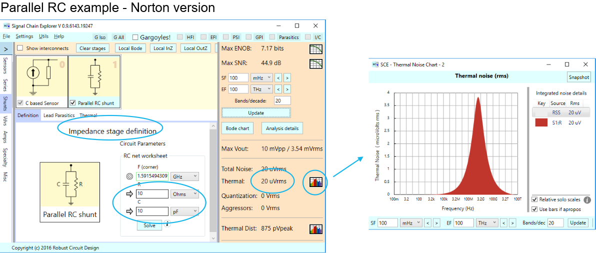
These results might seem surprising at first. All of the circuits have exactly same thermal noise, even down to the shape of the thermal noise plots themselves. Wow!

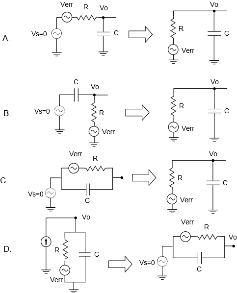
There’s a reason why this is so. As far as computing thermal noise referred-to-output is concerned, our circuit configurations all map to the same circuit — basically a parallel RC. We illustrate this below. In all of these circuits we set the voltage source to zero so that we can then find Verr referred to output (which is Vo).

Note that for the circuit involving the current source (D), we can convert it to its Thevenin equivalent, and see that it matches the circuit right above it (C). Thus, the current source version will have the same Verr referred to output.