Capacitor Impedance
In this Short and Sweet post, we take a brief look at how capacitors work and derive the formula for capacitor impedance, using Euler’s formula for complex exponentials. This post is a paraphrased excerpt from SWE Lesson 1.2.
A capacitor stores charge in the form of an electric field, or E-Field. In its most basic configuration it’s a pair of parallel plates, with an insulating material (or air, or vacuum) between them called the dielectric. When a voltage is applied across the plates, charges of opposite polarity accumulate on the plates, and an E-field develops.
Consider the following circuit, consisting of a battery, resistor, and capacitor, and a switch that allows the capacitor be charged and discharged.
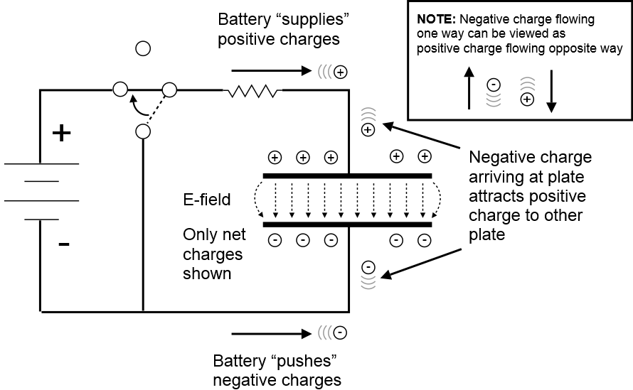
Suppose the capacitor is initially discharged (has no E-field), and then the switch is moved to connect the battery to the capacitor. Negative charges flow from the battery onto the lower plate of the capacitor, and these attract positive charges to the top plate. These positive charges can be thought of as negative charges (electrons) that have been displaced by leaving the top plate and returning to the battery. Thus a circuit is formed, and an E-field develops across the plate.
When a capacitor is charging (or discharging), there is charge flowing, and that means there is current. While you might think this means current flows through the capacitor, that is not the case, (at least not for an “ideal” capacitor). Charges move onto (or away) from the plates, but not across them. For this reason, the current associated with a capacitor is often called a displacement current.
A given capacitor can only hold so much charge, the amount being proportional to the voltage applied across the plates. The constant of proportionality is called the capacitance and the charge equation can be written as:
\(Q=CV\)
Since current is the time derivative of charge, we can derive a formula for the displacement current:
\(\displaystyle I(t)=\frac{{d{Q(t)}}}{{dt}} = C\frac{{dV(t)}}{{dt}}\)
We now have a relationship between voltage and current for a capacitor. If we take their ratio we can derive the capacitor’s impedance. The equation comes straight from Ohm’s Law:
\(\displaystyle Z = V / I\)
We’ve stated the equation generally, where each variable is complex. Here, Z is the impedance, and in general it’s a function of frequency. We treat V and I as being a function of frequency as well, and by making these variables complex rather than simple real numbers, we are able to represent this frequency dependence in an elegant way.
For the case of a capacitor, let’s see where Ohm’s Law takes us. We’ll start in the time domain. Assume V is a given. Then, since we know how I relates V through the capacitor current formula, we can write:
\(\displaystyle Z=\frac{V}{{C\frac{{dV}}{{dt}}}}\)
From the Land of Time to the Land of Frequency
How do we relate this differential equation, which is in the time domain, to the frequency domain? Well, here’s the trick: Suppose we think of our voltage as being sinusoidal (no, not suicidal, but sin-u-soid-al). That is, it’s some kind of sine or cosine wave. Let’s get even crazier and think of the voltage as being a complex sinusoid, having both imaginary and real parts.
Now why would we want to do this? Well, a long time ago, a particular formula was discovered that relates complex exponentials to complex sinusoids, and representing sinusoids as exponentials allows for a convenient, compact notation. That formula is known as Euler’s Formula:
\(\displaystyle A{{e}^{{j\theta }}}=A\cos \theta +jA\sin \theta\)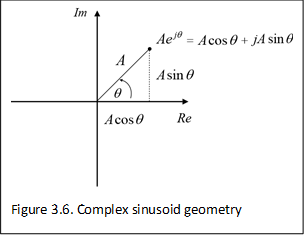
Might seem a bit bizarre, especially with the exponent of the exponential being complex, but maybe the figure on the right will aid in your understanding, as it shows the geometry in the complex plane.
You might wonder why we are introducing all this … er … complexity. (Pun intended). Patience, grasshopper.
We proceed by couching the voltage across the capacitor as a complex sinusoid, writing it as:
\(\displaystyle V(t)=A{{e}^{{j\omega t}}}=A\cos(\omega t)+jA\sin(\omega t)\)
where \(\omega\) is the frequency of the sinusoid, and \(\omega t = \theta\). Let’s plug that into our equation for current:
\(\displaystyle I(t)=C\frac{{dV(t)}}{{dt}}=C\frac{{d(A{{e}^{{j\omega t}}})}}{{dt}}=CA\frac{{d({{e}^{{j\omega t}}})}}{{dt}}=j\omega CA{{e}^{{j\omega t}}}\)
This algebra is taking advantage of the fact that the derivative of an exponential is just that same exponential, but with a scale factor in front. In short:
\(\displaystyle \frac{{d({{e}^{{kt}}})}}{{dt}}=k{{e}^{{kt}}}\)
For our case, \(k = j\omega\).
Now, let’s plug this into our formula for impedance. A funny thing happens when we do. A whole bunch of crap cancels out, and we end up with a simple (well, it’s actually complex, ha ha) expression for Z:
\(\require{cancel} \displaystyle Z=\frac{V}{I}=\frac{{A{{e}^{{j\omega t}}}}}{{j\omega CA{{e}^{{j\omega t}}}}}=\frac{{\cancel{{A{{e}^{{j\omega t}}}}}}}{{j\omega C\cancel{{A{{e}^{{j\omega t}}}}}}}=\frac{1}{{j\omega C}}\)
RC Filter Transfer Function
What can we do with the capacitor impedance formula? For one thing, we can derive the transfer function for a RC low pass filter. Here’s the circuit:
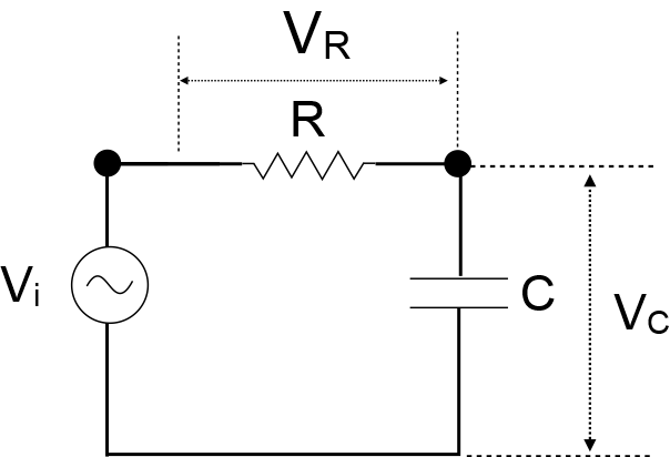
From the equation for voltage dividers we can write:
\(\displaystyle \frac{{Vc}}{{Vi}}=\frac{{{{Z}_{c}}}}{{R+{{Z}_{c}}}}=\frac{{1/(j\omega C)}}{{R+1/(j\omega C)}}\times \frac{{j\omega C}}{{j\omega C}}=\frac{1}{{j\omega RC+1}}\)
where \({Z}_{c}\) is the capacitor impedance. We can represent the output/input ratio in polar form, and write formulas for gain and phase: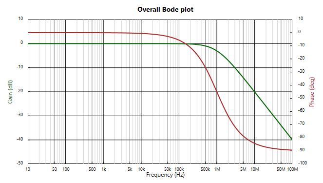
\(\displaystyle Gain(\omega )=\sqrt{{\frac{1}{{1+{{{(\omega RC)}}^{2}}}}}}\)
\(\displaystyle Phase(\omega )=-{{\tan }^{{-1}}}\left( {\frac{1}{{\omega RC}}} \right)\)
Plotted on a Bode chart, we get the classical low pass filter shape, here for a circuit with R = 159.2 Ohms, C = 1 nF:
Capacitor – Voltage Relation
We can use the complex exponential formula in another way that relates to capacitor impedance. We can see how voltage and current vary with respect to one another. You’ll see that, given a sine wave voltage, the capacitor current will be a cosine wave.
To derive this, we’ll take note of the following fact: The imaginary part of a complex exponential is a sine wave. To see this, let’s use our complex exponential formula for voltage:
\(\displaystyle Im[{{V}_{c}}(t)]=Im[A{{e}^{{j\omega t}}}]=Im[A\cos (\omega t)+jA\sin (\omega t)]=A\sin (\omega t)\)
So what about current? Well, to track the fact we’re using a sine wave voltage, which is the imaginary part of a complex exponential, we’ll take the imaginary part of the equation for current. So using our earlier formula for current, we can write:
\(\displaystyle Im[{{I}_{c}}(t)]=Im[j\omega CA{{e}^{{j\omega t}}}]=Im[j\omega CA(\cos (\omega t)+j\sin (\omega t))]\)
\(\displaystyle Im[{{I}_{c}}(t)]=Im[\omega CA(j\cos (\omega t)+{{j}^{2}}\sin (\omega t))]=Im[\omega CA(j\cos (\omega t)-\sin (\omega t)]\)
\(\displaystyle Im[{{I}_{c}}(t)]=\omega CAcos(\omega t)\)
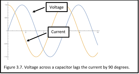
Comparing the voltage and current results, we arrive at an interesting fact: For a given sine wave voltage of amplitude A, the current is a cosine wave of amplitude \(\omega CA\).
Suppose A = 1V, \(\omega =1\,\,{{rad}}/{S}\;\), and C = 1 F. We plot both waveforms below. You’ll see that the capacitor voltage lags the current, or stated another way, the capacitor current leads the voltage:
Amazing what a little bit of math will do, especially when it involves complex exponentials.
Comments
Capacitor Impedance — No Comments
HTML tags allowed in your comment: <a href="" title=""> <abbr title=""> <acronym title=""> <b> <blockquote cite=""> <cite> <code> <del datetime=""> <em> <i> <q cite=""> <s> <strike> <strong>