Visualizing Noise in Signal Wave Explorer
Our new product Signal Wave Explorer will soon be ready for sale. It was a long and unexpected journey developing this product — unexpected because we weren’t quite sure when we started what the program would be capable of, and we kept getting surprised on the things it could do and what we could learn about signal processing.
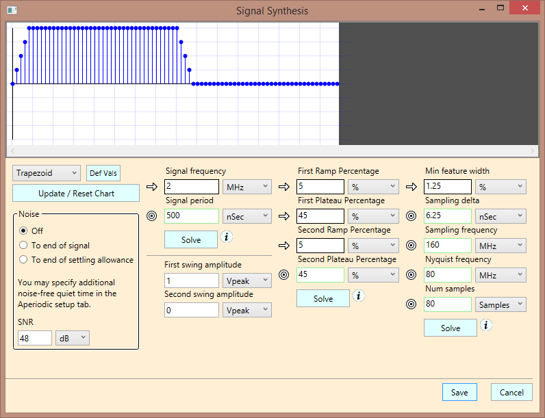
One of the exciting new features we’ve added is the ability to visualize thermal noise, (well, really, any type of Gaussian “white-noise.”) Here’s a clean, 2 MHz trapezoid signal with no noise, created using the Wave Definition Dialog of Signal Wave Explorer, using a sampling interval of 6.25 nS, for a sampling frequency of 160 MHz, and thus, 80 samples per trapezoid:
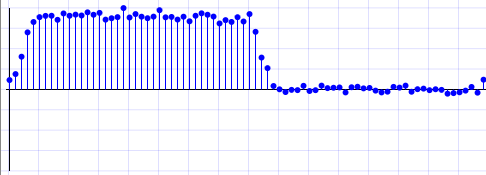
Notice the group box on the lower left corner. It’s here that you can add noise to the waveform, in terms of Signal to Noise Ratio (SNR). If you specify 48 dB SNR, select the “To end of signal” radio button, and press “Update”, then randomized noise (using Gaussian aka “normal” distribution) is added at a ratio of 251 parts signal to 1 part noise (48 dB) in terms of signal power. You end up with a wave looking something like:
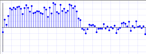
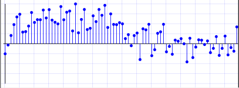
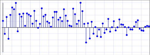
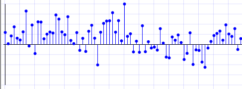
Here are other examples, using 24 dB, 10 dB, 0 dB, and even -6 dB SNR:
With this last example, you end up with a signal that doesn’t look anything like a trapezoid. But one of the cool things about signal processing is that if you know some properties of the signal, you can recover some semblance of it.
For example, suppose you are expecting a 2 MHz signal. You can add a 2 MHz “bandpass” filter in the form of a damped LRC filter, (damped using a resistor to prevent too much ringing, so admittedly it’s not much of a bandpass) and recover at least some aspects of the signal. Here’s an analog filter we quickly concocted in Signal Wave Explorer using the System Definition Dialog:
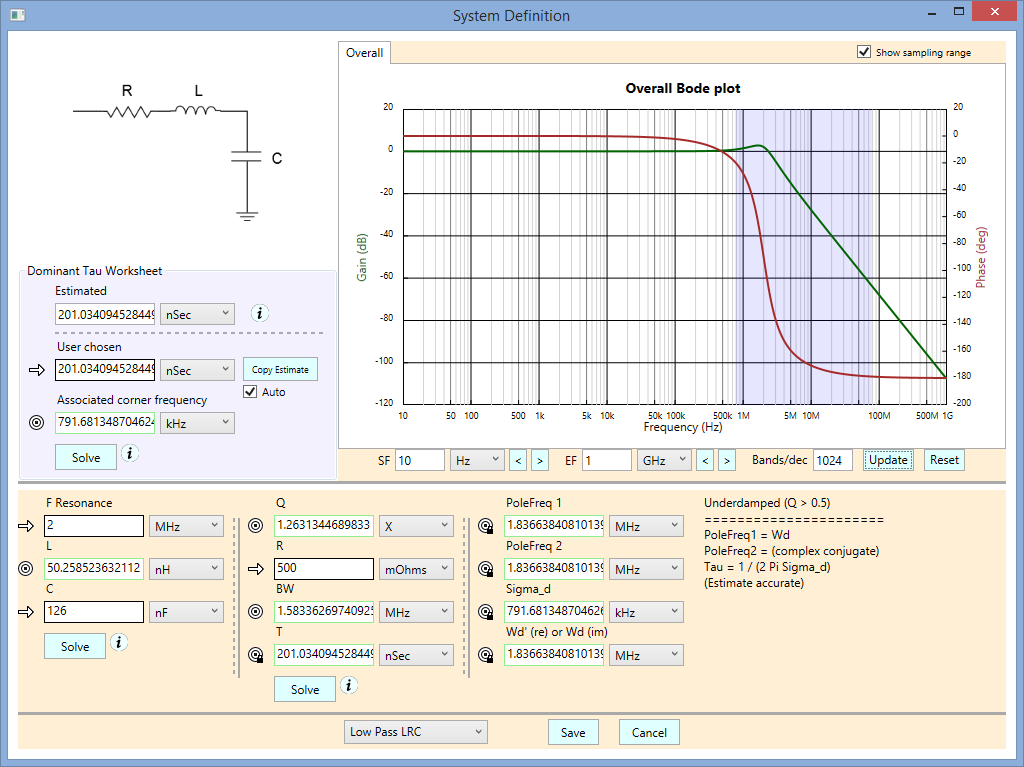 A filter to help isolate 2 MHz frequencies in the signal
Note the Bode chart, which shows the sampling range of our system in a light blue overlay. We can see that the peak is covered. Having this visual ability helps greatly in understanding what the sampling will do with our signal.
With Signal Wave Explorer, you can run a sampled simulation of our system, using multiple pulses of our signal, and see what you wrought. Here’s the main screen showing an example. The input wave is on the top. The output wave is on the bottom. In this example, we added eight noisy (-6 dB SNR) trapezoidal pulses. After the last pulse, we continue on for a while with the same level of noise energy that we had during the signal.
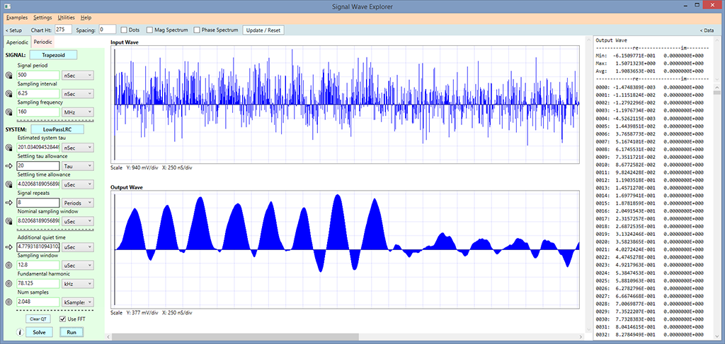
A simulation showing eight trapezoidal pulses with -6 dB SNR being filtered by an LRC filter.
In the output, you can clearly see that there were eight pulses present, though they are smoothed and distorted (and they go negative when they really shouldn’t — our trapezoids were unipolar.)
At any rate, this example illustrates some of the cool things you can do with Signal Wave Explorer. Version 1.0 is now complete and should be available for purchase in the next few days. So stay tuned!
If you wish to be notified when Signal Wave Explorer is ready for download, send us a note saying you want to be on our mailing list, and we’ll send you an email notification.
Comments
Visualizing Noise in Signal Wave Explorer — No Comments
HTML tags allowed in your comment: <a href="" title=""> <abbr title=""> <acronym title=""> <b> <blockquote cite=""> <cite> <code> <del datetime=""> <em> <i> <q cite=""> <s> <strike> <strong>